3D reconstruction

Using differentiable rendering to reconstuct volumes in DiffDRR

To perform 3D reconstruction with DiffDRR, we do the following:

1. Obtain target X-rays with corresponding camera poses (from the volume we wish to recover)
2. Initialize a moving DRR module with a random 3D volume
3. Measure the loss between the target X-ray and projections from the moving volume
4. Backpropogate this loss to the volume of the moving DRR and render from the new volume
5. Repeat Steps 3-4 until the loss has converged

1. Generate a target X-ray

import matplotlib.pyplot as plt
import torch
from tqdm import tqdm

from diffdrr.data import load_example_ct
from diffdrr.drr import DRR
from diffdrr.visualization import plot_drr

device = torch.device("cuda" if torch.cuda.is_available() else "cpu")

subject = load_example_ct()
drr = DRR(subject, sdd=1020.0, height=200, delx=2.0).to(device=device)

rotations = torch.tensor([[0.0, 0.0, 0.0]], device=device)
translations = torch.tensor([[0.0, 850.0, 0.0]], device=device)
gt = drr(rotations, translations, parameterization="euler_angles", convention="ZXY")
gt = (gt - gt.min()) / (gt.max() - gt.min())
plot_drr(gt, ticks=False)
plt.show()

2. Initialize a moving DRR from a random volume

Below is an implementation of a simple volume reconstruction module with DiffDRR.

Tip

As of v0.4.1, we can perform reconstruction with renderer="siddon". Note that for this to work, you have to use the default argument stop_gradients_through_grid_sample=True. For all prior versions of DiffDRR, you must use DRR(..., renderer="trilinear").

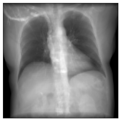
from diffdrr.pose import convert


class Reconstruction(torch.nn.Module):
    def __init__(self, subject, device):
        super().__init__()
        self.drr = DRR(subject, sdd=1020.0, height=200, delx=2.0).to(device=device)

        # Replace the known density with an initial estimate
        self.density = torch.nn.Parameter(
            torch.zeros(*subject.volume.spatial_shape, device=device)
        )

    def forward(self, pose, **kwargs):
        source, target = self.drr.detector(pose, None)
        source = self.drr.affine_inverse(source)
        target = self.drr.affine_inverse(target)
        img = self.drr.renderer(
            self.density,
            source,
            target,
            **kwargs,
        )
        return self.drr.reshape_transform(img, batch_size=len(pose))

3. Optimize!

• Render DRRs from the given camera poses
• Measure the loss between projected DRRs and the ground truth X-ray (here we use MSE)
• Update the estimate for the volume
• Repeat until converged!

recon = Reconstruction(subject, device)
optimizer = torch.optim.Adam(recon.parameters(), lr=1e-3)
criterion = torch.nn.MSELoss()

rotations = torch.tensor([[0.0, 0.0, 0.0]], device=device)
translations = torch.tensor([[0.0, 850.0, 0.0]], device=device)
pose = convert(
    rotations, translations, parameterization="euler_angles", convention="ZXY"
)

losses = []
for itr in tqdm(range(101), ncols=100):
    optimizer.zero_grad()
    est = recon(pose)
    loss = criterion(est, gt)
    loss.backward()
    optimizer.step()
    losses.append(loss.item())
    if itr % 25 == 0:
        plot_drr(
            torch.concat([est, gt, est - gt]),
            title=["Reconstruction", "Ground Truth", "Difference"],
        )
        plt.show()

plt.plot(losses)
plt.xlabel("# Iterations")
plt.ylabel("MSE")
plt.yscale("log")
plt.show()

  0%|                                                                       | 0/101 [00:00<?, ?it/s]

 25%|███████████████▎                                              | 25/101 [00:01<00:03, 21.13it/s]

 49%|██████████████████████████████                                | 49/101 [00:02<00:02, 21.02it/s]

 72%|████████████████████████████████████████████▊                 | 73/101 [00:04<00:01, 21.02it/s]

 99%|████████████████████████████████████████████████████████████▍| 100/101 [00:05<00:00, 21.25it/s]

100%|█████████████████████████████████████████████████████████████| 101/101 [00:05<00:00, 17.49it/s]

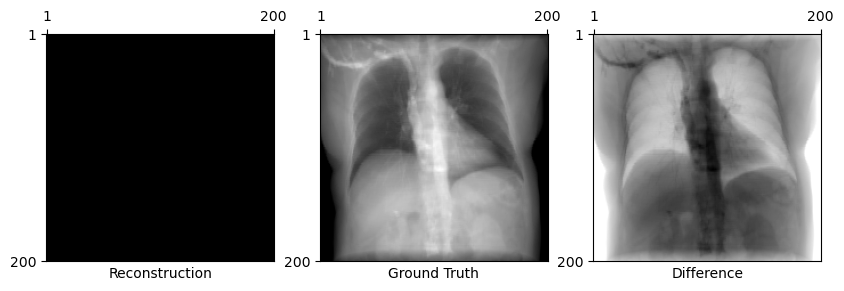
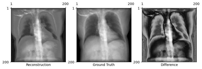
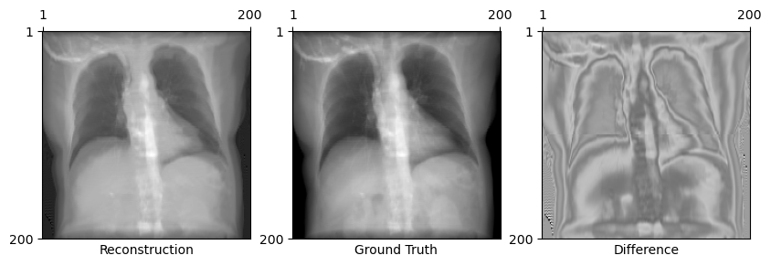
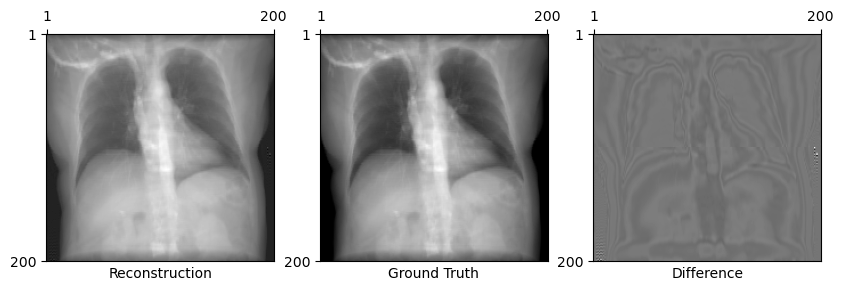
After optimizing for 100 iterations, we get a DRR that matches the input X-ray… even after starting with a randomly initialized voxelgrid! This demonstrates that differentiable rendering for volume reconstruction works with DiffDRR. But have we actually reconstructed something useful?

Novel view synthesis

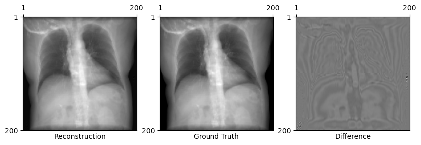
One way we can test the robustness of our reconstruction is by rendering DRRs from different poses.

First, let’s try bringing the C-arm 10 mm closer to the patient. Instantly, we can see that the intensities of the rendered images looks off…

rotations = torch.tensor([[0.0, 0.0, 0.0]], device=device)
translations = torch.tensor([[0.0, 840.0, 0.0]], device=device)
pose = convert(
    rotations, translations, parameterization="euler_angles", convention="ZXY"
)

plot_drr(
    torch.concat([recon(pose), drr(pose)]),
    title=["Reconstruction", "Ground Truth"],
)
plt.show()

Now let’s try rotating the detector by 1 degree. Issues are also very apparent here!

rotations = torch.tensor([[1.0, 0.0, 0.0]], device=device) / 180 * torch.pi
translations = torch.tensor([[0.0, 850.0, 0.0]], device=device)
pose = convert(
    rotations, translations, parameterization="euler_angles", convention="ZXY"
)

plot_drr(
    torch.concat([recon(pose), drr(pose)]),
    title=["Reconstruction", "Ground Truth"],
)
plt.show()

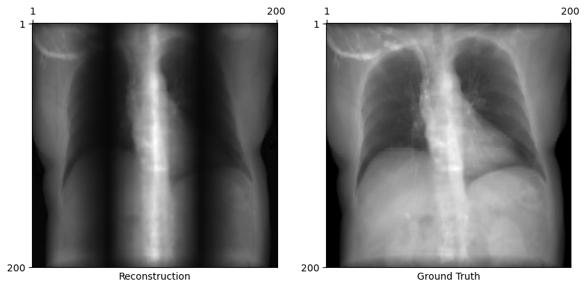
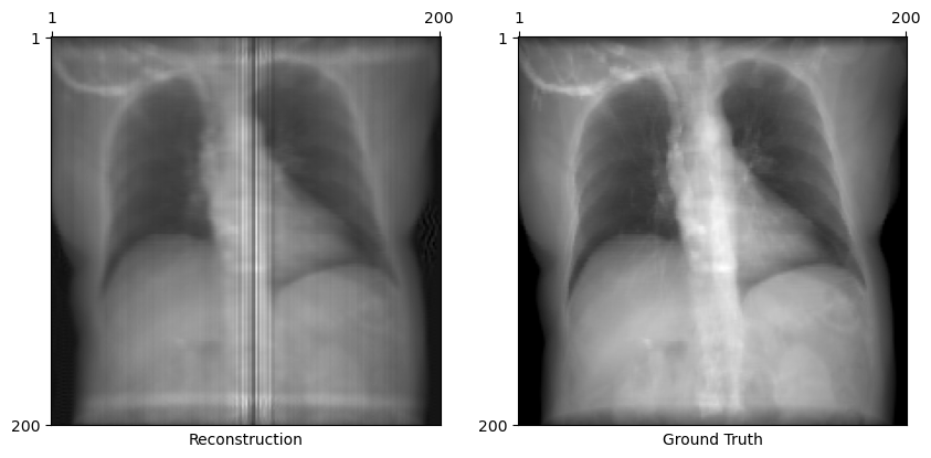
These results should not be surprising. After all, we were trying to reconstruct a 3D volume from a single X-ray. Real reconstruction algorithms typically require >100 images to achieve good novel view synthesis. Methods that achieve reconstruction with <100 images typically have some neural shenanigans going on (which one can totally do with DiffDRR!).

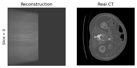
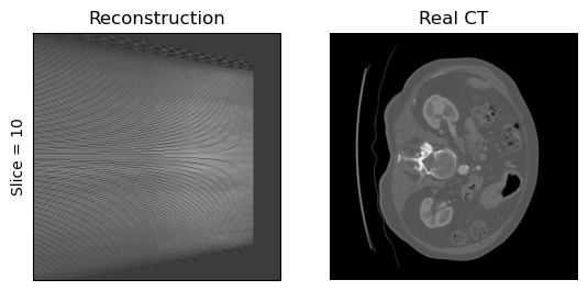
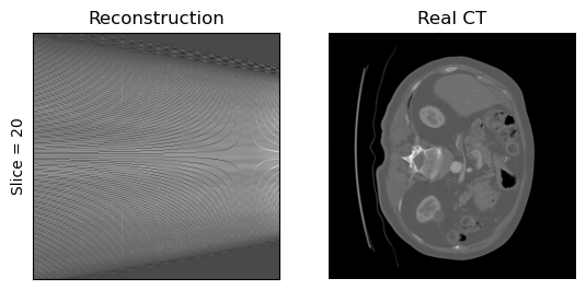
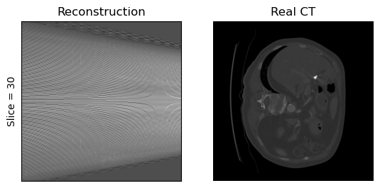
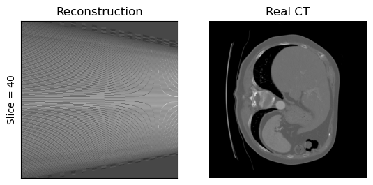
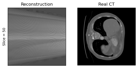
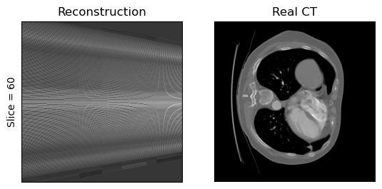
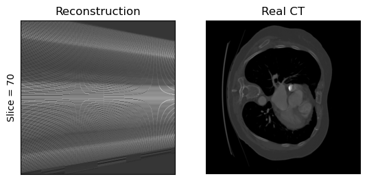
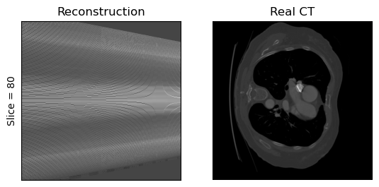
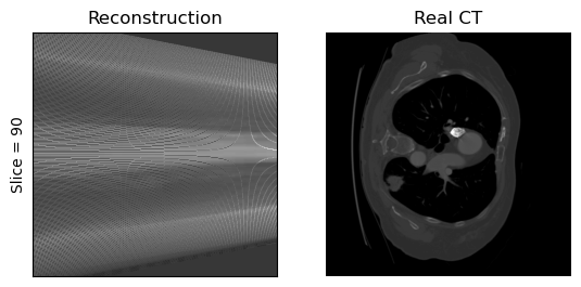
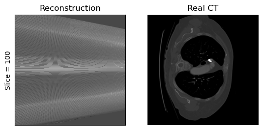
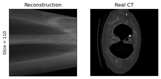
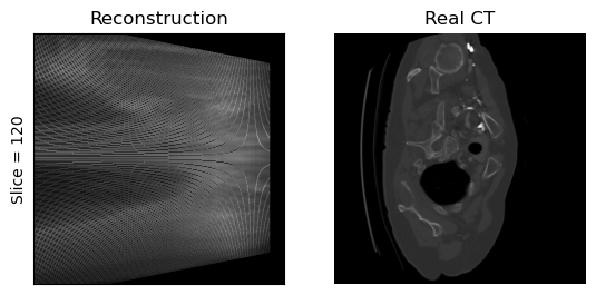
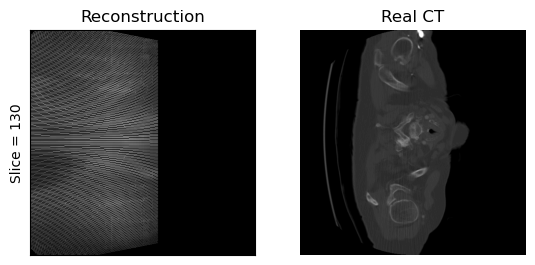
So what did we reconstruct?

We visualize slices from the volume reconstructed with DiffDRR and the original CT. The results are amusing! The takeaway is that the volume we reconstructed is incredibly overfit to produce the target X-ray. Every other X-ray that one might want to render is going to suffer horrible artifacts because our reconstruction isn’t generalized at all.

for jdx in range(0, 133, 10):
    plt.subplot(121)
    plt.imshow(recon.density[..., jdx].detach().cpu(), cmap="gray")
    plt.ylabel(f"Slice = {jdx}")
    plt.title("Reconstruction")
    plt.xticks([])
    plt.yticks([])
    plt.subplot(122)
    plt.imshow(drr.density[..., jdx].detach().cpu(), cmap="gray")
    plt.title("Real CT")
    plt.axis("off")
    plt.show()