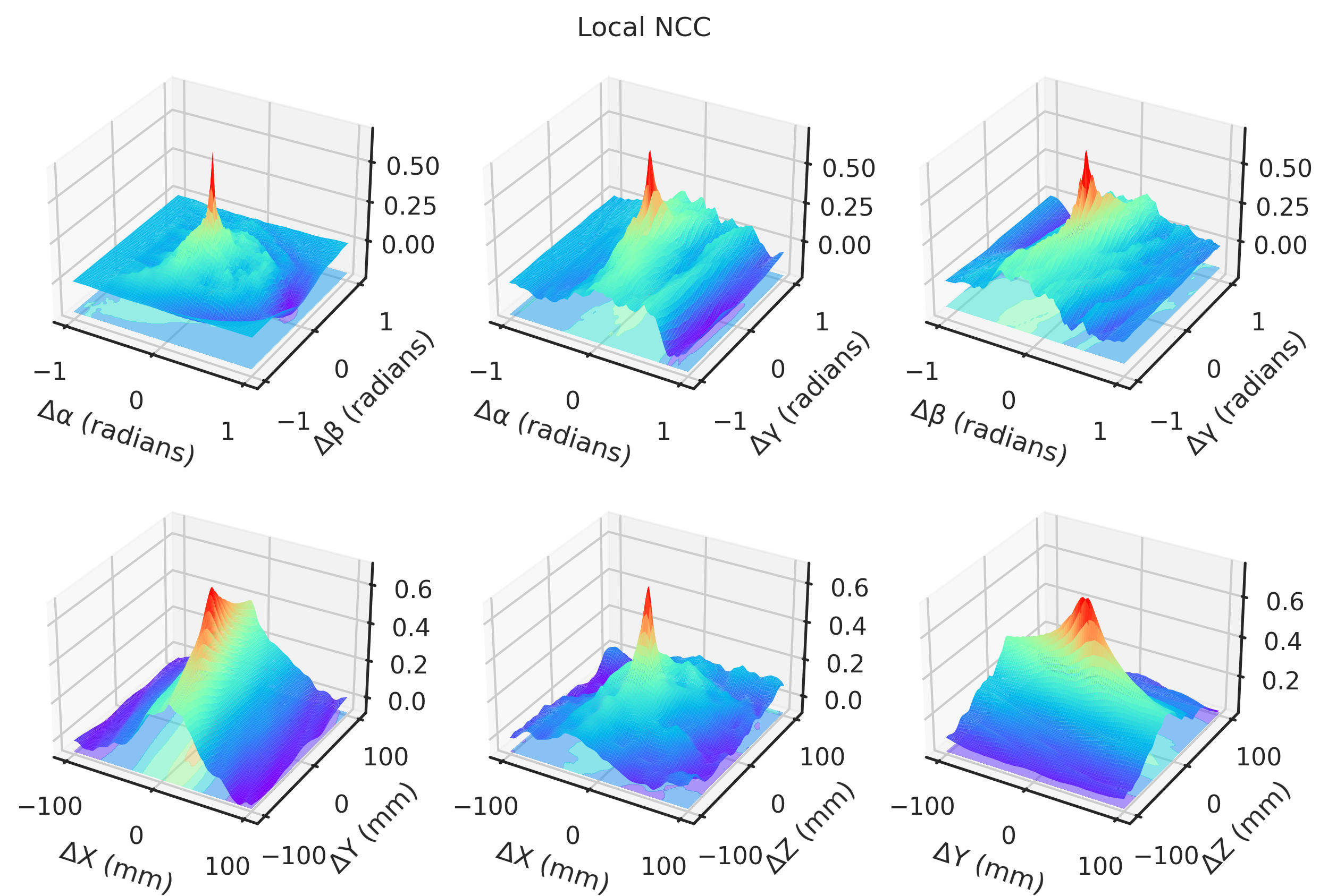
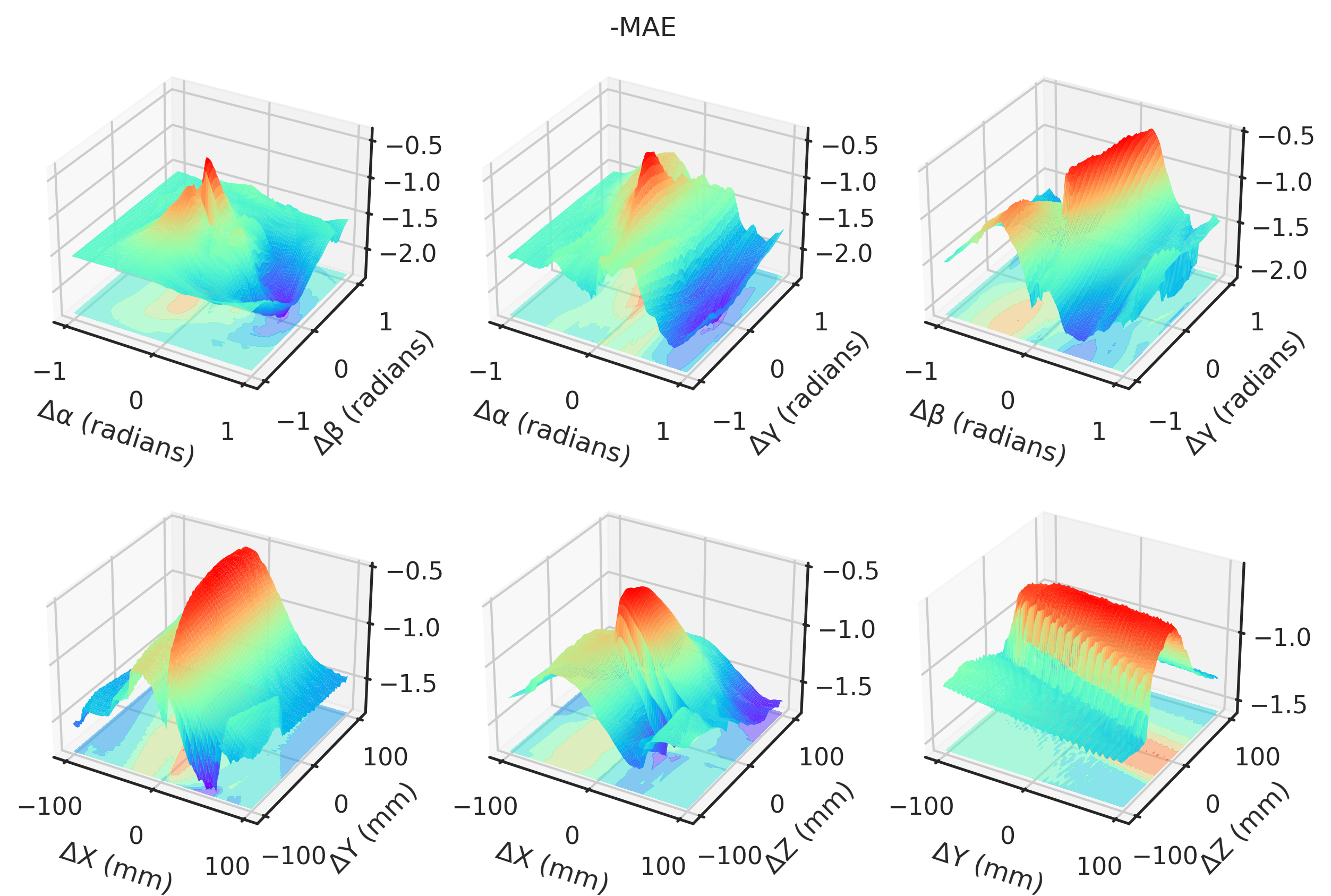
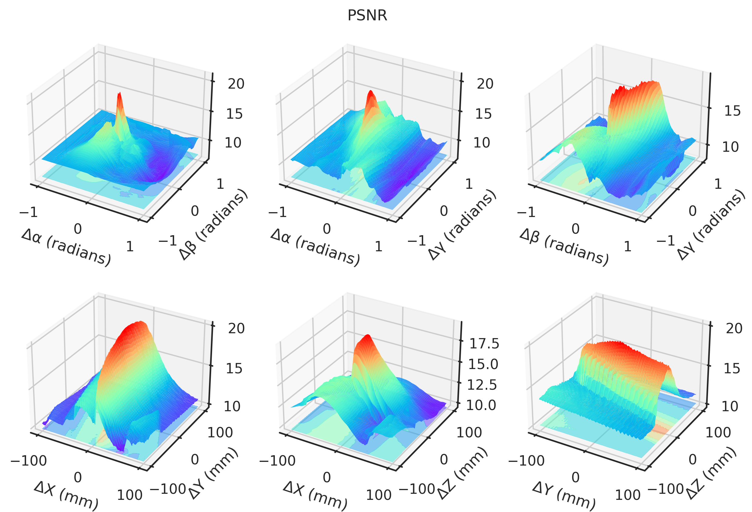
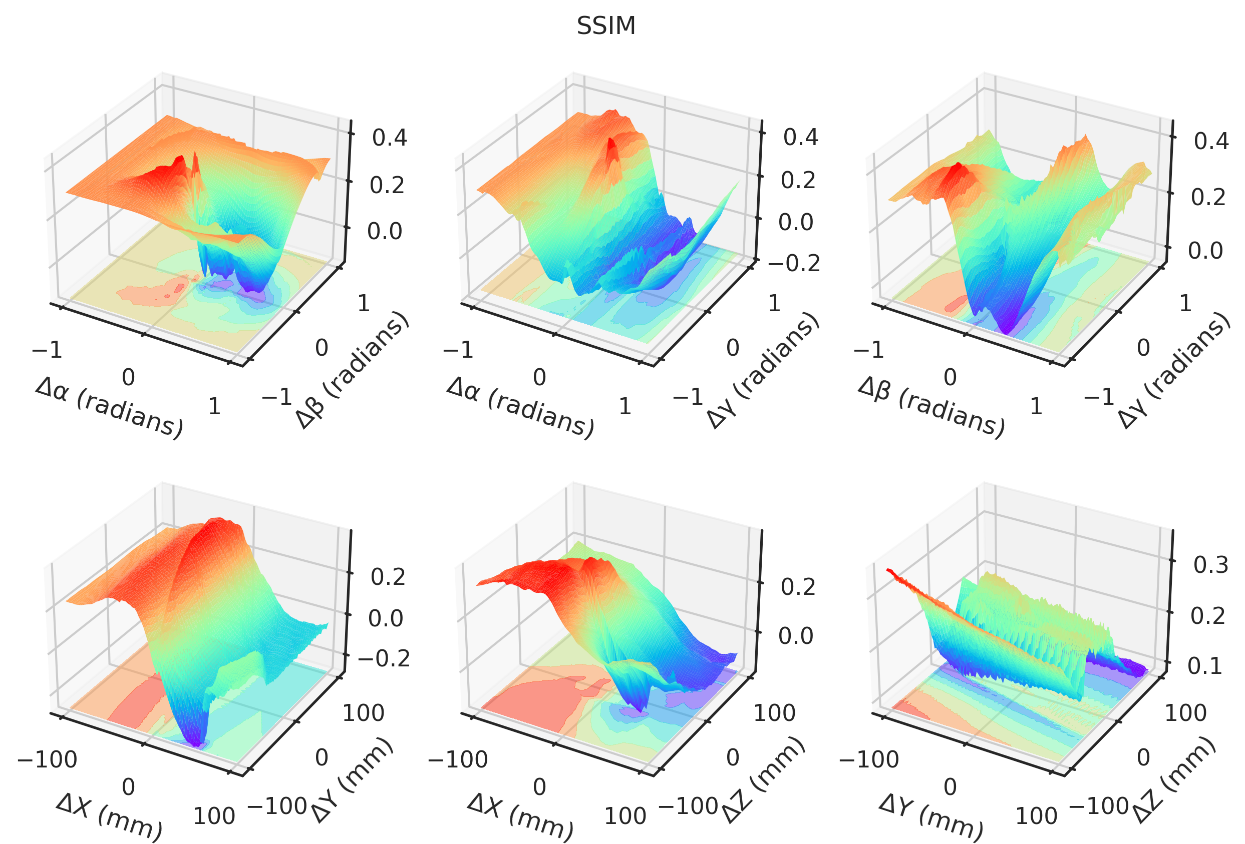
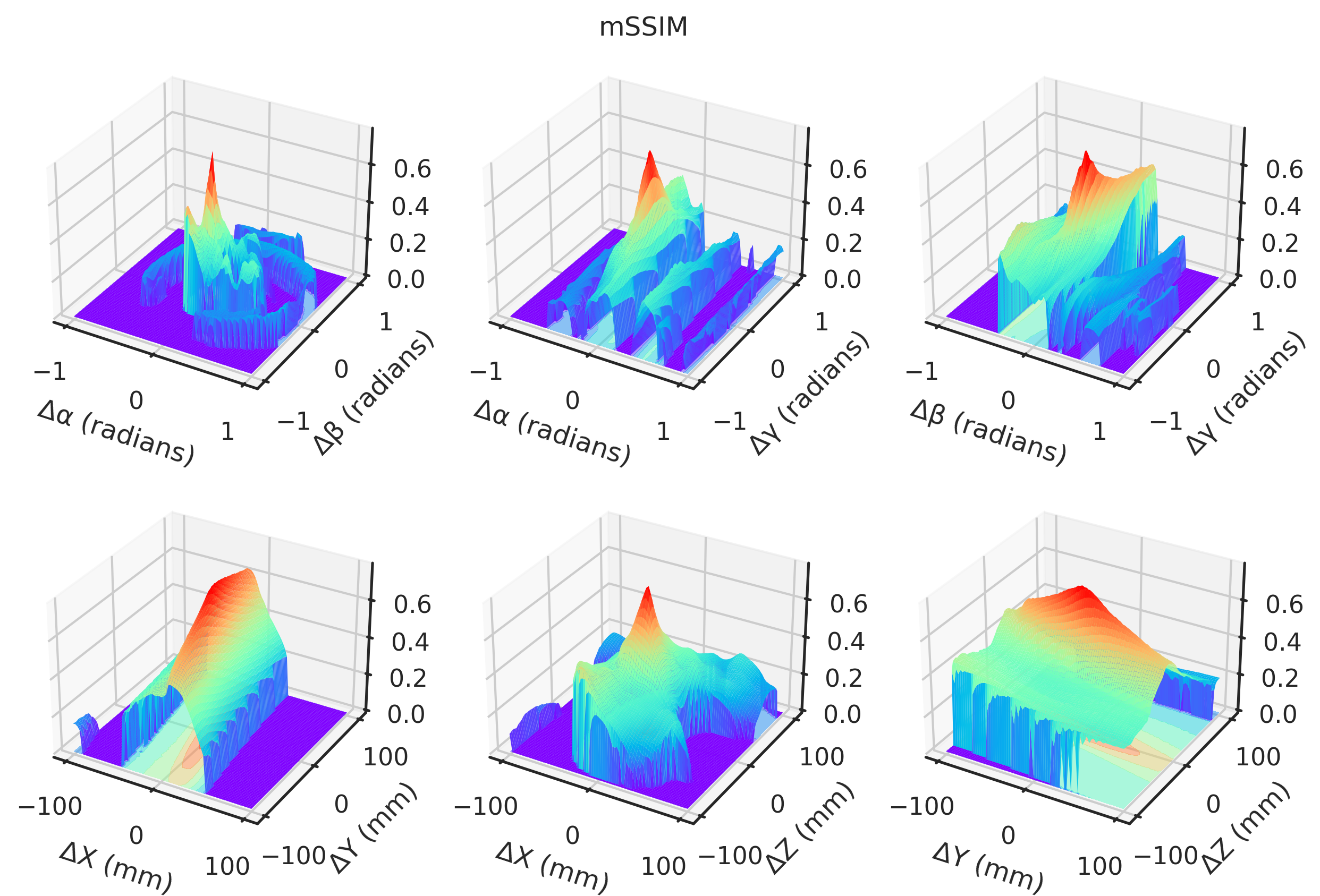
Visualizing loss landscapes

Images in the DeepFluoro dataset come with ground truth camera poses.

Images in the DeepFluoro dataset come with ground truth camera poses. By sampling simulated X-rays around the true pose, we can visualize the loss landscapes that we will have to optimize.

The metrics we try are

Mean Absolute Error
Mean Squared Error
Peak Signal-to-Noise Ratio
Structural Similarity Index Measure (SSIM)
Normalized Cross Correlation
Gradient Normalized Cross Correlation

If you want to try your own image similarity metric, implement it as a torchmetrics subclass.

Code

import matplotlib.pyplot as plt
import numpy as np
import seaborn
import torch
from diffdrr.drr import DRR
from diffdrr.utils import convert
from torchmetrics import MeanAbsoluteError, MeanSquaredError, MetricCollection
from torchmetrics.image import (
    MultiScaleStructuralSimilarityIndexMeasure,
    PeakSignalNoiseRatio,
    StructuralSimilarityIndexMeasure,
)
from torchvision.transforms.functional import center_crop, resize
from tqdm import tqdm

from diffpose.deepfluoro import DeepFluoroDataset, Transforms
from diffpose.metrics import (
    GradientNormalizedCrossCorrelation,
    MultiscaleNormalizedCrossCorrelation,
    NormalizedCrossCorrelation,
)


class Simulator(torch.nn.Module):
    def __init__(self, id_number, idx, subsample=8, **deep_fluoro_kwargs):
        super().__init__()
        self.specimen = DeepFluoroDataset(id_number, **deep_fluoro_kwargs)
        self.drr = self.setup_diffdrr(self.specimen, subsample)
        self.transforms = Transforms(size=self.height)

        true_xray, pose = self.specimen[idx]
        true_xray = self.transforms(true_xray)
        self.true_xray = true_xray.cuda()

        self.rotations = convert(
            pose.get_rotation(), "matrix", "euler_angles", None, "ZYX"
        ).cuda()
        self.translations = pose.get_translation().cuda()

    def setup_diffdrr(self, specimen, subsample):
        self.height = (1536 - 100) // subsample
        dx = 0.194 * subsample
        sdr = specimen.focal_len / 2
        return DRR(
            specimen.volume,
            specimen.spacing,
            sdr=sdr,
            height=self.height,
            delx=dx,
            x0=specimen.x0,
            y0=specimen.y0,
            reverse_x_axis=True,
            bone_attenuation_multiplier=2.5,
        ).cuda()

    def forward(
        self, rotations_offset=[0.0, 0.0, 0.0], translations_offset=[0.0, 0.0, 0.0]
    ):
        rotations = self.rotations + torch.tensor([rotations_offset]).cuda()
        translations = self.translations + torch.tensor([translations_offset]).cuda()
        pred_xray = self.drr(
            rotations, translations, parameterization="euler_angles", convention="ZYX"
        )
        pred_xray = self.transforms(pred_xray)
        return pred_xray, self.true_xray

simulator = Simulator(6, idx=1)
metrics = MetricCollection(
    {
        "MAE": MeanAbsoluteError(),
        "MSE": MeanSquaredError(),
        "PSNR": PeakSignalNoiseRatio(),
        "SSIM": StructuralSimilarityIndexMeasure(),
        "mSSIM": MultiScaleStructuralSimilarityIndexMeasure(),
        "NCC": NormalizedCrossCorrelation(),
        "LNCC": NormalizedCrossCorrelation(patch_size=13),
        "mNCC": MultiscaleNormalizedCrossCorrelation(
            patch_sizes=[13, None], patch_weights=[0.5, 0.5]
        ),
        "GNCC": GradientNormalizedCrossCorrelation(),
    }
).cuda()


def get_metrics(theta, phi, gamma, bx, by, bz):
    x, y = simulator([theta, phi, gamma], [bx, by, bz])
    m = metrics(x, y)
    return [v.item() for v in m.values()]

We search over a large capture range to visualize local minima:

Angular: ± 1 rad
Translation: ± 100 mm

# NCC for the angles
step = 0.025
t_angles = torch.arange(-1, 1.01, step=step)
p_angles = torch.arange(-1, 1.01, step=step)
g_angles = torch.arange(-1, 1.01, step=step)

# Get coordinate-wise correlations
tp_corrs = []
for t in tqdm(t_angles, ncols=50):
    for p in p_angles:
        xcorr = get_metrics(t, p, 0, 0, 0, 0)
        tp_corrs.append(xcorr)
TP = torch.tensor(tp_corrs).reshape(len(t_angles), len(p_angles), -1)

tg_corrs = []
for t in tqdm(t_angles, ncols=50):
    for g in g_angles:
        xcorr = get_metrics(t, 0, g, 0, 0, 0)
        tg_corrs.append(xcorr)
TG = torch.tensor(tg_corrs).reshape(len(t_angles), len(g_angles), -1)

pg_corrs = []
for p in tqdm(p_angles, ncols=50):
    for g in g_angles:
        xcorr = get_metrics(0, p, g, 0, 0, 0)
        pg_corrs.append(xcorr)
PG = torch.tensor(pg_corrs).reshape(len(p_angles), len(g_angles), -1)

100%|█████████████| 81/81 [03:18<00:00,  2.45s/it]
100%|█████████████| 81/81 [03:25<00:00,  2.53s/it]
100%|█████████████| 81/81 [03:22<00:00,  2.50s/it]

# NCC for the angles
step *= 100
xs = torch.arange(-100, 101, step=step)
ys = torch.arange(-100, 101, step=step)
zs = torch.arange(-100, 101, step=step)

# Get coordinate-wise correlations
xy_corrs = []
for x in tqdm(xs, ncols=50):
    for y in ys:
        xcorr = get_metrics(0, 0, 0, x, y, 0)
        xy_corrs.append(xcorr)
XY = torch.tensor(xy_corrs).reshape(len(xs), len(ys), -1)

xz_corrs = []
for x in tqdm(xs, ncols=50):
    for z in zs:
        xcorr = get_metrics(0, 0, 0, x, 0, z)
        xz_corrs.append(xcorr)
XZ = torch.tensor(xz_corrs).reshape(len(xs), len(zs), -1)

yz_corrs = []
for y in tqdm(ys, ncols=50):
    for z in zs:
        xcorr = get_metrics(0, 0, 0, 0, y, z)
        yz_corrs.append(xcorr)
YZ = torch.tensor(yz_corrs).reshape(len(ys), len(zs), -1)

100%|█████████████| 81/81 [03:21<00:00,  2.49s/it]
100%|█████████████| 81/81 [03:20<00:00,  2.47s/it]
100%|█████████████| 81/81 [03:20<00:00,  2.47s/it]

Plots and takeaways

Normalized Cross Correlation (Global NCC) appears to be the smoothest loss landscape
Local NCC (Local NCC) has the sharpest peak at the optimum, but has low gradients far from the optimum
Multiscale NCC (mNCC) achieves a good tradeoff between NCC and LNCC
Gradient NCC (Gradient NCC) is also peaked at the optimum, but has a difficult landscape further away
MAE, MSE, PSNR, SSIM, and mSSIM are inferior to NCC variants

Code

seaborn.set_theme(context="notebook", style="ticks")


def plot(idx, zmin=None, zmax=None):
    if idx == 2 or idx == 3:
        multiplier = -1
    else:
        multiplier = 1

    ### 3D
    fig = plt.figure(figsize=(10, 6.5), dpi=300)
    axs = []

    # Angles
    xyx, xyy = torch.meshgrid(t_angles, p_angles, indexing="ij")
    xzx, xzz = torch.meshgrid(t_angles, g_angles, indexing="ij")
    yzy, yzz = torch.meshgrid(p_angles, g_angles, indexing="ij")

    ax = fig.add_subplot(2, 3, 1, projection="3d")
    ax.contourf(
        xyx.numpy(),
        xyy.numpy(),
        multiplier * TP[..., idx].numpy(),
        zdir="z",
        offset=(multiplier * TP[..., idx]).min(),
        cmap=plt.get_cmap("rainbow"),
        alpha=0.5,
    )
    ax.plot_surface(
        xyx.numpy(),
        xyy.numpy(),
        multiplier * TP[..., idx].numpy(),
        rstride=1,
        cstride=1,
        cmap=plt.get_cmap("rainbow"),
        linewidth=0.0,
    )
    ax.set_xlabel("Δα (radians)")
    ax.set_ylabel("Δβ (radians)")
    ax.set_zlim3d(zmin, zmax)
    axs.append(ax)

    ax = fig.add_subplot(2, 3, 2, projection="3d")
    plt.title(
        [
            "Gradient NCC",
            "Local NCC",
            "-MAE",
            "-MSE",
            "Global NCC",
            "PSNR",
            "SSIM",
            "mNCC",
            "mSSIM",
        ][idx]
    )
    ax.contourf(
        xzx.numpy(),
        xzz.numpy(),
        multiplier * TG[..., idx].numpy(),
        zdir="z",
        offset=(multiplier * TG[..., idx]).min(),
        cmap=plt.get_cmap("rainbow"),
        alpha=0.5,
    )
    ax.plot_surface(
        xzx.numpy(),
        xzz.numpy(),
        multiplier * TG[..., idx].numpy(),
        rstride=1,
        cstride=1,
        cmap=plt.get_cmap("rainbow"),
        linewidth=0.0,
    )
    ax.set_xlabel("Δα (radians)")
    ax.set_ylabel("Δγ (radians)")
    ax.set_zlim3d(zmin, zmax)
    axs.append(ax)

    ax = fig.add_subplot(2, 3, 3, projection="3d")
    ax.contourf(
        yzy.numpy(),
        yzz.numpy(),
        multiplier * PG[..., idx].numpy(),
        zdir="z",
        offset=(multiplier * PG[..., idx]).min(),
        cmap=plt.get_cmap("rainbow"),
        alpha=0.5,
    )
    ax.plot_surface(
        yzy.numpy(),
        yzz.numpy(),
        multiplier * PG[..., idx].numpy(),
        rstride=1,
        cstride=1,
        cmap=plt.get_cmap("rainbow"),
        linewidth=0.0,
    )
    ax.set_xlabel("Δβ (radians)")
    ax.set_ylabel("Δγ (radians)")
    ax.set_zlim3d(zmin, zmax)
    axs.append(ax)

    # Angles
    xyx, xyy = torch.meshgrid(xs, ys, indexing="ij")
    xzx, xzz = torch.meshgrid(xs, zs, indexing="ij")
    yzy, yzz = torch.meshgrid(ys, zs, indexing="ij")

    ax = fig.add_subplot(2, 3, 4, projection="3d")
    ax.contourf(
        xyx.numpy(),
        xyy.numpy(),
        multiplier * XY[..., idx],
        zdir="z",
        offset=(multiplier * XY[..., idx]).min(),
        cmap=plt.get_cmap("rainbow"),
        alpha=0.5,
    )
    ax.plot_surface(
        xyx.numpy(),
        xyy.numpy(),
        multiplier * XY[..., idx].numpy(),
        rstride=1,
        cstride=1,
        cmap=plt.get_cmap("rainbow"),
        linewidth=0.0,
    )
    ax.set_xlabel("ΔX (mm)")
    ax.set_ylabel("ΔY (mm)")
    ax.set_zlim3d(zmin, zmax)
    axs.append(ax)

    ax = fig.add_subplot(2, 3, 5, projection="3d")
    ax.contourf(
        xzx.numpy(),
        xzz.numpy(),
        multiplier * XZ[..., idx].numpy(),
        zdir="z",
        offset=(multiplier * XZ[..., idx]).min(),
        cmap=plt.get_cmap("rainbow"),
        alpha=0.5,
    )
    ax.plot_surface(
        xzx.numpy(),
        xzz.numpy(),
        multiplier * XZ[..., idx].numpy(),
        rstride=1,
        cstride=1,
        cmap=plt.get_cmap("rainbow"),
        linewidth=0.0,
    )
    ax.set_xlabel("ΔX (mm)")
    ax.set_ylabel("ΔZ (mm)")
    ax.set_zlim3d(zmin, zmax)
    axs.append(ax)

    ax = fig.add_subplot(2, 3, 6, projection="3d")
    ax.contourf(
        yzy.numpy(),
        yzz.numpy(),
        multiplier * YZ[..., idx].numpy(),
        zdir="z",
        offset=(multiplier * YZ[..., idx]).min(),
        cmap=plt.get_cmap("rainbow"),
        alpha=0.5,
    )
    ax.plot_surface(
        yzy.numpy(),
        yzz.numpy(),
        multiplier * YZ[..., idx].numpy(),
        rstride=1,
        cstride=1,
        cmap=plt.get_cmap("rainbow"),
        linewidth=0.0,
    )
    ax.set_xlabel("ΔY (mm)")
    ax.set_ylabel("ΔZ (mm)")
    ax.set_zlim3d(zmin, zmax)
    axs.append(ax)

    return fig, axs

plot(0)
plt.show()

plot(1)
plt.show()

plot(2)
plt.show()

plot(3)
plt.show()

plot(4)
plt.show()

plot(5)
plt.show()

plot(6)
plt.show()

plot(7)
plt.show()

plot(8)
plt.show()